Big O, Big Θ, Big Ω¶

What You'll Learn

✅ What asymptotic notation is and why we need it
✅ The difference between Big O (upper bound), Big Ω (lower bound), and Big Θ (tight bound)
✅ How to read and write complexity expressions
✅ The most common complexity classes and what they feel like at scale
✅ How to determine which notation to use when analysing an algorithm
✅ Common misconceptions and traps

When we analyse an algorithm, we don't care about exact runtimes — those depend on hardware, language, and input quirks. Instead, we ask: how does the runtime grow as input size grows? Asymptotic notation gives us a precise mathematical language to answer that question.

New to Complexity Analysis?

Start by thinking of Big O as a speed limit sign — it tells you the worst it can get, not how fast you're going right now. Once that clicks, Big Θ and Big Ω fall into place naturally.

Already know the basics?

Focus on the Formal Definitions and Choosing the Right Notation sections — most developers use these terms loosely and mix them up in interviews.

Keep in mind

In everyday conversation (and most interviews), people say "Big O" when they really mean Big Θ (tight bound). Knowing the difference matters for technical accuracy — and for impressing interviewers.

The Three Notations at a Glance¶

graph LR
    A["f(n) — actual runtime"] --> B["Big O: f(n) = O(g(n))\nUpper bound\n'at most this bad'"]
    A --> C["Big Ω: f(n) = Ω(g(n))\nLower bound\n'at least this good'"]
    A --> D["Big Θ: f(n) = Θ(g(n))\nTight bound\n'exactly this order'"]

    style B fill:#ff6b6b,color:#fff
    style C fill:#51cf66,color:#fff
    style D fill:#339af0,color:#fff

1️⃣ Why Asymptotic Notation?¶

Consider two sorting algorithms:

# Algorithm A: always does exactly 3n² + 5n + 12 operations
# Algorithm B: always does exactly 100n + 200 operations

n = 10:     A = 362 ops      B = 1,200 ops   → A wins
n = 100:    A = 30,512 ops   B = 10,200 ops   → B wins
n = 1,000:  A = 3,005,012    B = 100,200      → B wins by 30x
n = 1,000,000: A ≈ 3×10¹²   B ≈ 10⁸          → B wins by 30,000x

The growth rate of the dominant term is what matters at scale. We drop constants and lower-order terms:

3n² + 5n + 12  →  O(n²)    (quadratic growth dominates)
100n + 200     →  O(n)     (linear growth dominates)

The golden rule

Drop constants. Drop lower-order terms. Keep only the fastest-growing term.

5n³ + 2n² + 100n + 9  →  O(n³)
n log n + n            →  O(n log n)
42                     →  O(1)

2️⃣ The Complexity Classes¶

Complexity growth rate chart Growth rate comparison of common complexity classes — HackerEarth

Class	Name	Example
O(1)	Constant	Array index access, hash map lookup
O(log n)	Logarithmic	Binary search, balanced BST ops
O(n)	Linear	Linear search, single loop
O(n log n)	Linearithmic	Merge sort, heap sort
O(n²)	Quadratic	Bubble sort, nested loops
O(n³)	Cubic	Naive matrix multiplication
O(2ⁿ)	Exponential	Recursive Fibonacci, subset generation
O(n!)	Factorial	Permutation generation, brute-force TSP

3️⃣ Formal Definitions¶

Big O — Upper Bound¶

f(n) = O(g(n)) means there exist positive constants c and n₀ such that: f(n) ≤ c · g(n) for all n ≥ n₀

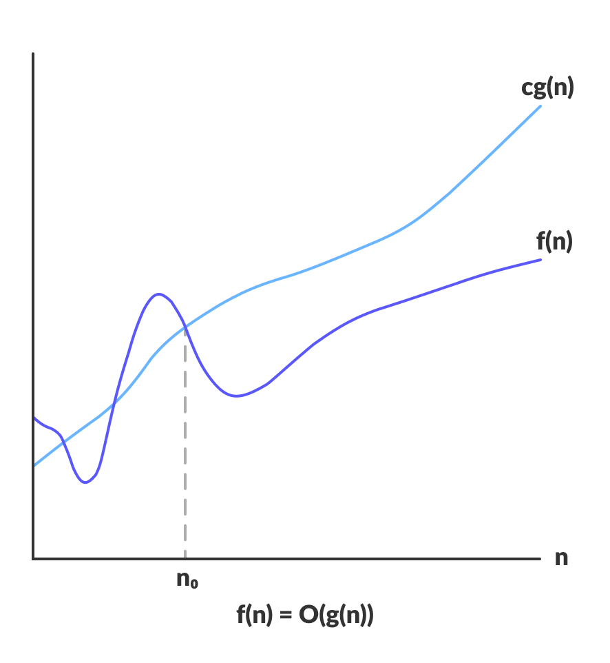Big O upper bound diagram f(n) stays below c·g(n) for all n past n₀ — source: Programiz

Example: f(n) = 3n + 5 - Choose c = 4, n₀ = 5: 3n + 5 ≤ 4n for all n ≥ 5 ✅ - Therefore: f(n) = O(n)

Big Ω — Lower Bound¶

f(n) = Ω(g(n)) means there exist positive constants c and n₀ such that: f(n) ≥ c · g(n) for all n ≥ n₀

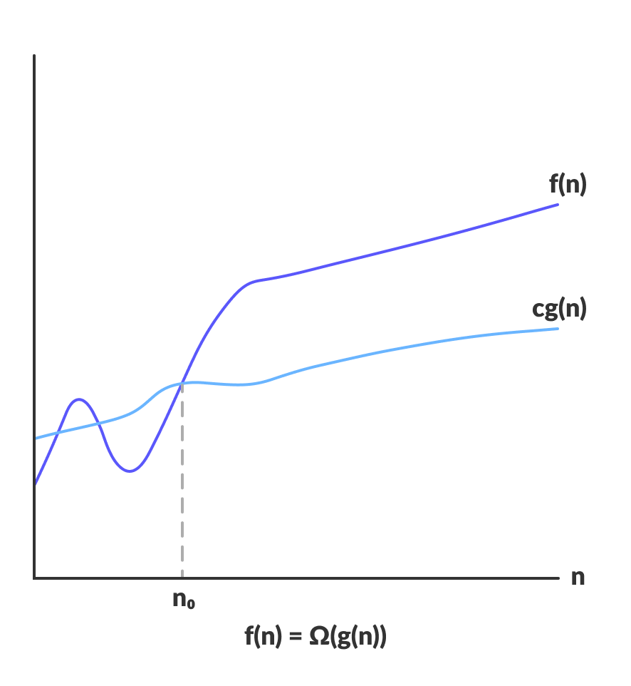Big Omega lower bound diagram f(n) stays above c·g(n) for all n past n₀ — source: Programiz

Example: Any comparison-based sort is Ω(n log n) — you can't do better than that in the worst case.

Big Θ — Tight Bound¶

f(n) = Θ(g(n)) means f(n) = O(g(n)) AND f(n) = Ω(g(n))

Equivalently: there exist constants c₁, c₂, n₀ such that: c₁ · g(n) ≤ f(n) ≤ c₂ · g(n) for all n ≥ n₀

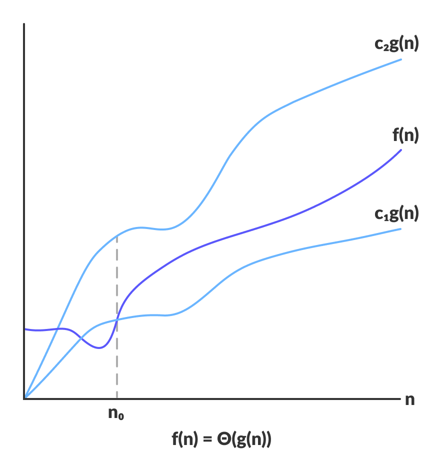Big Theta tight bound diagram f(n) is sandwiched between c₁·g(n) and c₂·g(n) for all n past n₀ — source: Programiz

Example: f(n) = 3n + 5 = Θ(n) because it's both O(n) and Ω(n).

4️⃣ Big O in Code¶

O(1) — ConstantO(log n) — LogarithmicO(n) — LinearO(n log n) — LinearithmicO(n²) — Quadratic

def get_first(lst):
    return lst[0]        # one operation, regardless of list size

def is_even(n):
    return n % 2 == 0    # one operation

def binary_search(arr, target):
    lo, hi = 0, len(arr) - 1
    while lo <= hi:
        mid = (lo + hi) // 2
        if arr[mid] == target:
            return mid
        elif arr[mid] < target:
            lo = mid + 1    # discard left half
        else:
            hi = mid - 1    # discard right half
    return -1
# Each iteration halves the search space → log₂(n) iterations

def find_max(lst):
    max_val = lst[0]
    for item in lst:      # visits each element once
        if item > max_val:
            max_val = item
    return max_val

def merge_sort(arr):
    if len(arr) <= 1:
        return arr
    mid = len(arr) // 2
    left = merge_sort(arr[:mid])   # log n levels of recursion
    right = merge_sort(arr[mid:])
    return merge(left, right)      # O(n) work at each level
# log n levels × O(n) merge = O(n log n)

def bubble_sort(arr):
    n = len(arr)
    for i in range(n):          # outer loop: n iterations
        for j in range(n - 1):  # inner loop: n iterations
            if arr[j] > arr[j + 1]:
                arr[j], arr[j + 1] = arr[j + 1], arr[j]
# n × n = n² comparisons in the worst case

5️⃣ Analysing Cases: Best, Average, Worst¶

An algorithm can behave differently depending on the input. We analyse three cases:

def linear_search(lst, target):
    for i, val in enumerate(lst):
        if val == target:
            return i    # found — stop early
    return -1

Case Analysis for Linear Search
──────────────────────────────────────────────────────
  Best case    →  target is lst[0]   →  1 comparison   →  Ω(1)
  Average case →  target is in middle → n/2 comparisons → Θ(n)
  Worst case   →  target not in list →  n comparisons   →  O(n)
──────────────────────────────────────────────────────
  Big O  describes the WORST case upper bound
  Big Ω  describes the BEST case lower bound
  Big Θ  describes the TIGHT bound (when best ≈ worst)
──────────────────────────────────────────────────────

O and Ω are bounds, not cases

This is one of the most common confusions. Big O is not the worst case — it's an upper bound. You can correctly say linear_search = O(n²) (it's true but loose). Big O just says "it won't grow faster than this." The tight worst-case bound is Θ(n).

6️⃣ Simplification Rules¶

# Rule 1: Drop constants
O(3n)     →  O(n)
O(500)    →  O(1)
O(2n²)   →  O(n²)

# Rule 2: Drop lower-order terms
O(n² + n)       →  O(n²)
O(n log n + n)  →  O(n log n)
O(2ⁿ + n¹⁰⁰)   →  O(2ⁿ)

# Rule 3: Sequential steps → ADD
def two_loops(n):
    for i in range(n):    # O(n)
        pass
    for j in range(n):    # O(n)
        pass
# Total: O(n) + O(n) = O(2n) → O(n)

# Rule 4: Nested steps → MULTIPLY
def nested_loops(n):
    for i in range(n):        # O(n)
        for j in range(n):    # O(n)
            pass
# Total: O(n) × O(n) = O(n²)

# Rule 5: Different inputs → different variables
def two_arrays(a, b):
    for x in a:    # O(a)
        pass
    for y in b:    # O(b)
        pass
# Total: O(a + b)  ← NOT O(n), they're separate inputs!

Sequential vs Nested

The + vs × distinction is critical. Sequential loops add; nested loops multiply. This single rule explains why two nested loops over n items is O(n²), not O(2n).

7️⃣ Choosing the Right Notation¶

Use Big O when...Use Big Ω when...Use Big Θ when...

You want to give a guarantee — the algorithm will not be worse than this.

Reporting worst-case performance to stakeholders
Comparing algorithms where the worst case matters (e.g. real-time systems)
Most interview and textbook contexts — it's the default notation

# Insertion sort: O(n²) worst case
# Even if the input is sorted (O(n) best case), we guarantee O(n²)

You want to give a lower bound — no algorithm can do better than this.

Proving theoretical limits: "any comparison sort requires Ω(n log n)"
Showing a problem is inherently hard
Proving your algorithm is optimal

# Searching an unsorted array: Ω(n)
# You MUST look at every element — no shortcut exists

You know both the upper and lower bound — the exact growth order.

When best and worst cases have the same growth rate
Precise academic analysis
Describing algorithms that behave consistently

# Merge sort: Θ(n log n) — always, regardless of input
# Binary search: Θ(log n) — always halves the space

8️⃣ Common Traps and Misconceptions¶

# ❌ Trap 1: O(n) doesn't mean "fast"
# O(n) with n = 10⁹ is still a billion operations.
# Constants matter in practice even if we drop them theoretically.

# ❌ Trap 2: Confusing Big O with worst case
# These are independent. Big O is a bound, not a case.
# Quicksort is O(n²) worst case, but also O(n log n) average case.
# Both statements use Big O for different scenarios.

# ❌ Trap 3: Same variable for different inputs
def func(a, b):
    for x in a:      # this is O(|a|), not O(n)
        for y in b:  # this is O(|b|), not O(n)
            pass
# Correct: O(|a| × |b|)  — NOT O(n²) unless |a| == |b|

# ❌ Trap 4: Ignoring space complexity
# Big O applies to space too, not just time.
# Recursive functions use O(depth) call stack space.
def factorial(n):
    if n == 0: return 1
    return n * factorial(n - 1)
# Time: O(n), Space: O(n) — each call lives on the stack

Space complexity

Every call to a recursive function uses stack space. factorial(n) creates n stack frames before any returns — so it's O(n) space even though it looks simple. Iterative versions are O(1) space.

9️⃣ Practical Complexity Targets¶

Input Size → Acceptable Complexity
──────────────────────────────────────────────────────
  n ≤ 10        →  O(n!), O(2ⁿ)     fine
  n ≤ 20        →  O(2ⁿ)             fine
  n ≤ 100       →  O(n³)             fine
  n ≤ 1,000     →  O(n²)             fine
  n ≤ 100,000   →  O(n log n)        fine
  n ≤ 10⁶       →  O(n)              fine
  n ≤ 10⁸       →  O(log n), O(1)    fine
──────────────────────────────────────────────────────
Rule of thumb: 10⁸ simple operations ≈ 1 second in Python

Interview strategy

When asked to optimise, work backwards from the input size. If n ≤ 10⁵, you need at most O(n log n). If O(n²) is your current solution, that's your target to beat.

🔟 Side-by-Side Summary¶

Notation   Symbol   Bound     Says...                      Example
─────────────────────────────────────────────────────────────────────────
Big O      O(g(n))  Upper     "grows no faster than g(n)"  3n+5 = O(n)
Big Omega  Ω(g(n))  Lower     "grows no slower than g(n)"  3n+5 = Ω(1)
Big Theta  Θ(g(n))  Tight     "grows at exactly g(n)"      3n+5 = Θ(n)
─────────────────────────────────────────────────────────────────────────
  If f(n) = Θ(g(n)), then BOTH f(n) = O(g(n)) AND f(n) = Ω(g(n))
  The reverse is NOT always true.
─────────────────────────────────────────────────────────────────────────

✅ Quick Reference Summary¶

Notation	Meaning	Analogy	When to use
O(g(n))	Upper bound — at most this	Speed limit (won't exceed)	Worst-case guarantees, interviews
Ω(g(n))	Lower bound — at least this	Minimum time required	Proving theoretical limits
Θ(g(n))	Tight bound — exactly this	Precise measurement	When algorithm is consistent
O(1)	Constant time	Instant	Array access, hash lookup
O(log n)	Logarithmic	Halving the problem	Binary search, tree height
O(n)	Linear	One pass	Single loop, linear scan
O(n log n)	Linearithmic	Sort-then-scan	Merge sort, heap sort
O(n²)	Quadratic	Nested loops	Bubble sort, brute force pairs
O(2ⁿ)	Exponential	Doubles per step	Recursive backtracking
O(n!)	Factorial	All permutations	Brute-force TSP